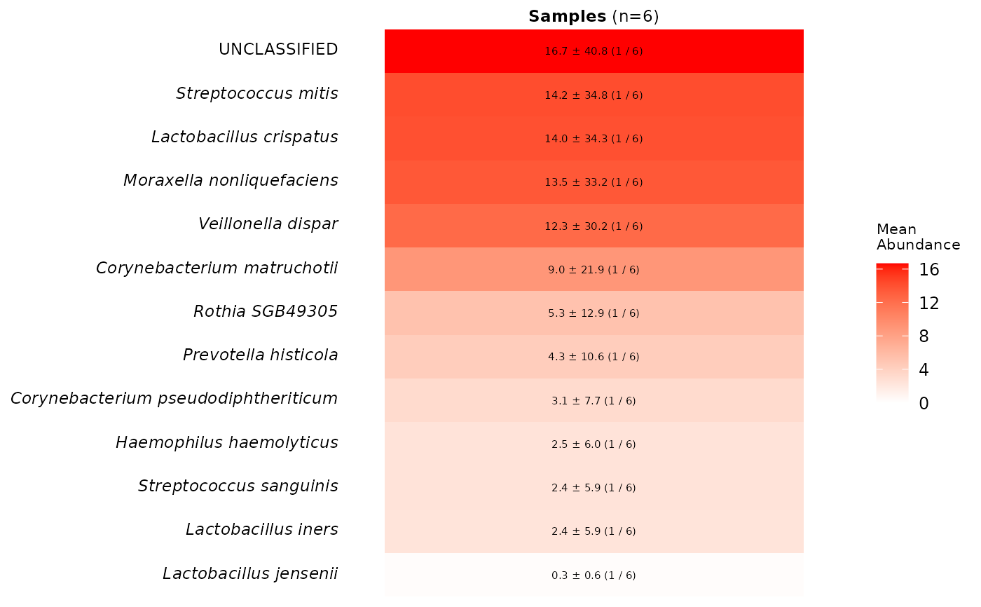
Creates a ggplot2-based heatmap that displays either mean abundance or prevalence of taxa in its gradient across samples or sample groups. It helps identify dominant or prevalent taxa and visualize patterns possibly influenced by experimental factors. Text labels within cells display mean abundance ± SD and prevalence.
Usage
plot_taxa_heatmap(
  me,
  tax_rank,
  group_var = NULL,
  plot_title = NULL,
  group_labels = NULL,
  color_by = c("abundance", "prevalence"),
  prevalence_display = c("percent", "fraction"),
  order_by = c("abundance", "prevalence", "alphabetical"),
  min_abundance = 0,
  min_prevalence = 0,
  as_relative = TRUE,
  filter_by_group = FALSE,
  ...
)
Arguments
- me
A
microEDAorphyloseqobject containing OTU and taxonomic data.- tax_rank
Characterstring specifying taxonomic rank (e.g., "Genus", "Family"). Abbreviations (e.g., "g") are allowed.- group_var
(Optional)
Characterstring indicating a sample variable to group samples. IfNULL, all samples are treated as one group.- plot_title
(Optional)
Characterstring for the plot title.- group_labels
(Optional) Named character vector to rename group levels (e.g.,
c("Old" = "New")).- color_by
Character. What to color the tiles by:"abundance"(mean abundance) or"prevalence".- prevalence_display
Character. Display prevalence as"percent"(e.g., 75%) or"fraction"(e.g., 6/8).- order_by
Character. Order taxa by"abundance"(mean abundance),"prevalence", or"alphabetical".- min_abundance
Numericvalue. Minimum abundance threshold for a feature to be retained. Must be non-negative. Features with abundance below this are considered absent.- min_prevalence
Numericvalue. Minimum prevalence required for retention. If value is < 1, interpreted as proportion of samples; otherwise, as absolute number of samples.- as_relative
Logical. IfTRUE, applies relative abundance transformation (TSS) to the input counts. IfFALSE, uses raw counts. (Default:TRUE).- filter_by_group
Logical. IfFALSE(default), filtering is applied globally across all samples even ifgroup_varis specified. This allows usinggroup_varfor stratification in plotting without affecting the filtering scope. IfTRUE, filtering is applied within each group defined bygroup_varandgroup_requirement. See filter_features for more details on filtering arguments.- ...
Additional arguments for fine-tuning. Can include:
k:Integer. Number of decimal places for label formatting (Default: 1).font_size:Numericvalue. Font size for text labels heatmap cells (Default: 2).legend_text: Font size for legend (Default: 9).legend_key: Size/height of legend (Default: 15).ntaxa: Number of top taxa to display (Default: 30).abundance_criterion:Characterstring. Criterion to use for filtering:prevalence:Retain features present in at least
min_prevalencesamples (within group ifgroup_varis used) and with abundance >=min_abundancein those samples.mean:Also requires that the mean abundance across samples (or group) is >=
min_abundance.
Default:
"prevalence".group_requirement:Characterstring. Whengroup_varis specified, determines whether the filter criterion must be met in"any"group or"all"groups. Default:"any".keep_filtered: Whether to keep filtered out taxa as "Other" (Default:TRUE). Takes effect only formicroEDAobjects.rm_missing:Logical.IfTRUE, removes taxa with missing/unclassified entries at the specified rank. IfFALSE, fills missing values by propagating the last known ancestor, labeling them as "Unclassified Last_Known_Parent_Clade" (e.g., "Unclassified Enterobacteriaceae"). (Default:FALSE).process_taxon: Whether to clean taxon names (remove underscores, return in italic). (Default:TRUE).low_color,high_color: Colours for low and high ends of the gradient. (Default:"white"and"red")
Details
The function prepares the taxonomic profile by:
Filtering taxa by
min_abundance,min_prevalence.Aggregating counts by
tax_rank.Reducing the total number of taxa to no more than
ntaxa.Optionally applies relative abundance transformation (TSS) to the data.
If
group_varis specified, samples are grouped by that variable.Sample counts per group are appended to group labels (e.g., "Control (n=10)").
The value used for coloring (color_by) and the value used for ordering
(order_by) can be specified independently. Text labels within cells display
mean abundance ± SD and prevalence.
Examples
mpa <- microEDA(merged_metaphlan_profiles)
plot_taxa_heatmap(mpa, "Species", prevalence_display = "fraction")
#> Warning: Both 'min_abundance' and 'min_prevalence' are 0. No filtering will be applied.
#> Plotting data...